模具管理中有生產績效報表，進度報表、產能負荷報表、機臺負荷報表等等，將數據進行分組匯總后，看到的數據還是不夠直觀，所以要進行圖表的建立。如果要生成每個模號的圖表。

第一種方式：建立模板文件，將數據復制進去即可形成圖表，這里的前提是分組的數據要用公式先設置好，如果分組是動態的，或者不顯示零值的數據。那么就要采用第二種方式。

第二種方式：通過取數據庫數據，然后在excel菜單中點擊按鈕進行拉取數據，過濾處理后，然后進行分組統計，最后顯示數據和圖表，這樣數據是最新格式，可按程序指令進行格式處理，保證數據的準確安全。并且運行速度是最快的。

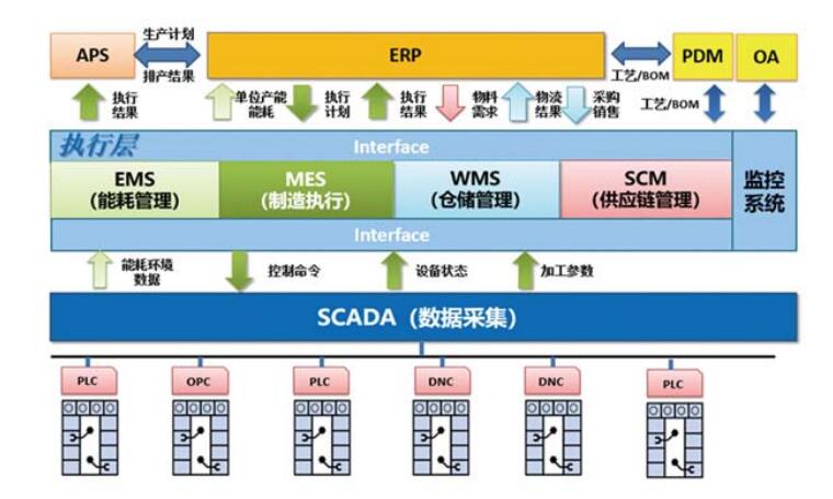
云易云軟件基于數據庫管理系統，Excel相結合的方式進行模具管理與生產績效報表分析。Excel的便捷在于，報表的深度加工處理，很多管理系統都無法調整到個性化級別。以及報表電子檔方式發送到客戶供應商。對于上游客戶需要進行產量、質量報備的情況下。數據庫與VBA代碼可提供管理信息系統的改造，實現企業的生態化管理。

以下為生成圖表的源碼，有問題可咨詢QQ：53757591

Private Sub 生成圖表(ByVal sh As String, ByVal a1 As Integer, ByVal a2 As Integer, ByVal tol As Long)
Dim mychart As String
Dim i As Integer
ActiveWindow.ScrollRow = 1
ActiveWindow.ScrollColumn = 1
    Charts.Add
    mychart = ActiveChart.Name
    ActiveChart.ApplyCustomType ChartType:=xlBuiltIn, TypeName:="兩軸線-柱圖"
    ActiveChart.SetSourceData Source:=Sheets(sh).Range("A65536"), PlotBy _
        :=xlColumns
    ActiveChart.SeriesCollection.NewSeries
    ActiveChart.SeriesCollection.NewSeries
    ActiveChart.SeriesCollection(1).XValues = "='" & sh & "'!R" & a1 & "C2:R" & a2 & "C2"
    ActiveChart.SeriesCollection(1).Values = "='" & sh & "'!R" & a1 & "C3:R" & a2 & "C3"
    ActiveChart.SeriesCollection(2).Values = "='" & sh & "'!R" & a1 & "C9:R" & a2 & "C9"
    ActiveChart.Location where:=xlLocationAsObject, Name:=sh
    ActiveChart.ApplyCustomType ChartType:=xlBuiltIn, TypeName:="兩軸線-柱圖"
    With ActiveChart
        .HasTitle = False
        .Axes(xlCategory, xlPrimary).HasTitle = True
        .Axes(xlCategory, xlPrimary).AxisTitle.Characters.Text = "不良項目"
        .Axes(xlValue, xlPrimary).HasTitle = True
        .Axes(xlValue, xlPrimary).AxisTitle.Characters.Text = "不良數"
        .Axes(xlCategory, xlSecondary).HasTitle = False
        .Axes(xlValue, xlSecondary).HasTitle = True
        .Axes(xlValue, xlSecondary).AxisTitle.Characters.Text = "累積影響度"
    End With
    ActiveChart.HasLegend = False
    ActiveChart.Axes(xlValue).AxisTitle.Select
    With Selection
        .HorizontalAlignment = xlCenter
        .VerticalAlignment = xlCenter
        .ReadingOrder = xlContext
        .Orientation = xlVertical
    End With
    ActiveChart.Axes(xlValue, xlSecondary).AxisTitle.Select
    With Selection
        .HorizontalAlignment = xlCenter
        .VerticalAlignment = xlCenter
        .ReadingOrder = xlContext
        .Orientation = xlVertical
    End With
    ActiveChart.Axes(xlValue).Select
    With ActiveChart.Axes(xlValue)
        .MinimumScale = 0
        .MaximumScale = tol
        .MinorUnit = 4
        .MajorUnit = tol / 5
        .Crosses = xlAutomatic
        .ReversePlotOrder = False
        .ScaleType = xlLinear
        .DisplayUnit = xlNone
    End With
    ActiveChart.Axes(xlValue, xlSecondary).Select
    With ActiveChart.Axes(xlValue, xlSecondary)
        .MinimumScale = 0
        .MaximumScale = 100
        .MinorUnit = 25
        .MajorUnit = 25
        .Crosses = xlAutomatic
        .ReversePlotOrder = False
        .ScaleType = xlLinear
        .DisplayUnit = xlNone
    End With
    ActiveChart.SeriesCollection(1).Select
    With Selection.Border
        .Weight = xlThin
        .LineStyle = xlAutomatic
    End With
    Selection.Shadow = False
    Selection.InvertIfNegative = False
    Selection.Interior.ColorIndex = xlNone
    With ActiveChart.ChartGroups(1)
        .Overlap = 0
        .GapWidth = 0
        .HasSeriesLines = False
        .VaryByCategories = False
    End With
    ActiveChart.PlotArea.Select
    With Selection.Border
        .ColorIndex = 16
        .Weight = xlThin
        .LineStyle = xlContinuous
    End With
    Selection.Interior.ColorIndex = xlNone
    For i = 1 To ActiveSheet.ChartObjects.Count
        ActiveSheet.ChartObjects(i).Select
        ActiveChart.ChartArea.Select
        ActiveSheet.Shapes(i).Left = Range("J31").Left
        ActiveSheet.Shapes(i).Top = Range("J31").Top
        ActiveSheet.Shapes(i).Width = Range("S43").Left - Range("J31").Left
        ActiveSheet.Shapes(i).Height = Range("S43").Top - Range("J31").Top
    Next i
End Sub